I built a RAG system in 48 hours.

Introduction

In our life as engineers, the use of LLMs has become increasingly unavoidable. Whether for drafting assistance, reverse engineering, or even development, it is a game-changer tool whose adoption in daily life is no longer in doubt. This technology is part of the continuity of major revolutions that have multiplied our capabilities, like the arrival of the personal computer or universal access to the Internet.

However, this poses a problem of sovereignty and control we have over these tools: where is the data we send recorded? For what purposes is it used? There is no doubt in my mind that for many ChatGPT users, the application often knows them better than the people around them. And even beyond these considerations, we create a dependency, through our daily use of these tools, on the platforms that manage them. What will prevent them in the future from multiplying their price by 2? By 3? These are phenomena far from fiction, which are happening in the Cloud industry. Many large accounts, having migrated to Cloud Providers (Azure, GCP, AWS...), find themselves crushed by rates over which they are gradually losing control.

What conclusions should be drawn? From my point of view, we must not fall into the demonization of these tools and completely reject them. They remain formidable assets when used well. But it is also an opportunity in my opinion to open the hood of these services, understand how they work to better use them, and above all be able to do without them if necessary. It's a bit like knowing how to navigate without GPS: we use it for comfort, but we keep the ability to find our way if the signal disappears.

It is for these reasons that I wanted to challenge myself: would it be possible, in 48h, to deploy a reliable solution locally?

[Day 1] Preparations

The first step consists of creating a corpus, a bibliography. In my case, I decided to retrieve "founding" documents in the world of Machine Learning.

• Leo Breiman, 1996, Bagging Predictors
• Leo Breiman, 2001, Random Forests
• Corinna Cortes & Vladimir Vapnik, 1995, Support-Vector Networks
• Yoav Freund & Robert E. Schapire, 1997, A Decision-Theoretic Generalization of On-Line Learning and an Application to Boosting
• Jerome H. Friedman, 2001, Greedy Function Approximation: A Gradient Boosting Machine
• Trevor Hastie, Robert Tibshirani & Jerome Friedman, 2009, The Elements of Statistical Learning: Data Mining, Inference, and Prediction
• Alex Krizhevsky, Ilya Sutskever & Geoffrey E. Hinton, 2012, ImageNet Classification with Deep Convolutional Neural Networks
• Yann LeCun, Léon Bottou, Yoshua Bengio & Patrick Haffner, 1998, Gradient-Based Learning Applied to Document Recognition
• David E. Rumelhart, Geoffrey E. Hinton & Ronald J. Williams, 1986, Learning Representations by Back-Propagating Errors
• Vladimir Vapnik & Alexey Chervonenkis, 1971, On the Uniform Convergence of Relative Frequencies of Events to Their Probabilities

These documents represent 233 pages of scientific articles and 750 pages for Hastie's book. This will constitute a first corpus sufficient for testing. I also write a file in bibtex format to fill in the metadata of each document.

I then install Ollama, a tool through which it is possible to download local LLMs and run a server that will transmit our chat requests to them. I take the Llama3 model, the version with 8 billion parameters. I launch it, I ask it a question. My GPU gets busy, and, after a few seconds: my answer is there!

For the moment, nothing very impressive, but there is still a small satisfaction in running the model locally.

[Day 1] The RAG Architecture.

This is where we get a little more into the details of the RAG architecture. The initial question is: when a user formulates a prompt, how to select the most relevant sources?

First, are we obliged to select? The answer is yes. Each LLM is capable of working with more or less rich contexts: we speak of context window, expressed in number of tokens. In a simplified way, we can consider that 1 token = 1 word.

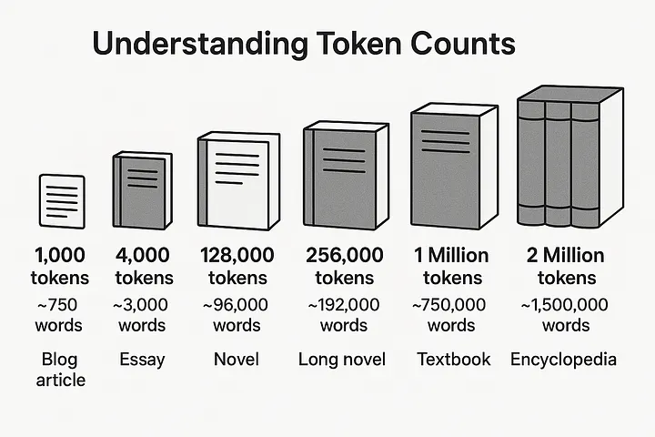
In our case, the Llama3:8B that I am running is capable of handling 8000 tokens, which represents about 10 pages of scientific articles. Problem: I have articles of much more than 10 pages in my corpus. And I have a book of 750 pages... To get around this, we will prepare our data upstream, so that it can be exploited during the generation of the response. There is no exact science at this stage but an example of a solution can look like this:

For each .pdf document:

1. Extract the text.
2. Clean it, retrieve graph data (The non-trivial task detector activates here :) )
3. Format the result in structured Markdown, which is an ideal format when conversing with LLMs.
4. Cutting .md files into chunks of length 1000, with a certain overlap (so as not to lose context if we cut a sentence in two). These values are what are called hyperparameters of the RAG.

• Note: Each chunk inherits metadata from the document it comes from: this will allow us to find the origin of information.

5. Mystery step 1 which will be addressed later.
6. Mystery step 2 which will, also, be addressed later.

The slicing into chunks will allow the system to digest a much larger amount of information. Like in cooking when you cut a potato into cubes before cooking it. For the rest we therefore work with chunks, document dice.

In order to evaluate the relevance of each chunk with respect to the question asked by the user, a similarity score is calculated. This score calculation brings up a new element in the RAG architecture: the embedding.

Embedding is the encoding of data with the aim of positioning them in an N-dimensional space: a bit like giving each chunk GPS coordinates. It is then enough to calculate the GPS coordinates of the user's question to be able to evaluate the geographical distance between the two: the closer it is, the more similarity there is between the chunk (and therefore the document it comes from) and the user prompt.

My explanation hides (fascinating) complexity but the logic is indeed this one.

That said, the embedding process is costly and is therefore not done on the fly, especially since the GPS coordinates of our chunks do not change from one embedding to another. So we need at this stage a way to save the information locally: this is where ChromaDB comes into play. It is a vector database optimized for storing and querying embeddings. It allows for example to search for elements by semantic similarity instead of having precise criteria as one might have with a classic SQL DBMS. This allows us to say "return me the k nearest neighbors of this vector that I give you".

Here are unsurprisingly the mystery steps that were hidden behind steps 5 & 6:

5. Embedding of each chunk using an Encoder (which by the way is done by an ML model)
6. Recording of "GPS Coordinates", which are actually vectors, in ChromaDB, with indexing to accelerate read access to this information.

Here is a diagram that summarizes all the elements I talked about.

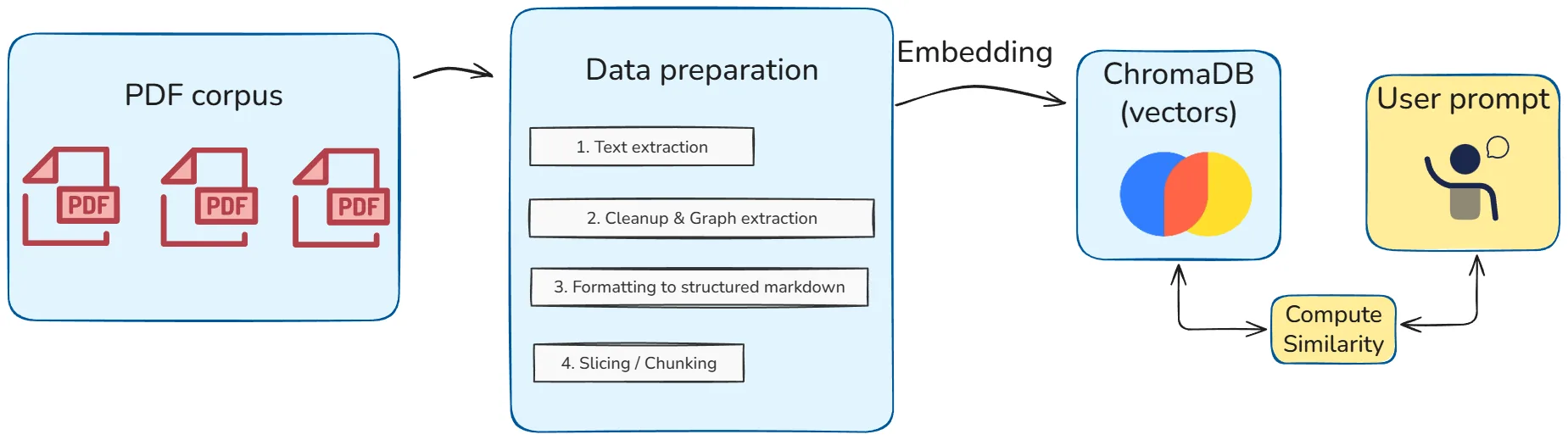
I simplified it to the maximum but it covers the fundamental steps of the system that I will have to put in place.

[Day 1] Implementation.

At this stage no line of code had yet been written. It was necessary to remedy this, time playing against me.

I decide to split the project into modules each responsible for a part of the system. We will therefore have:

• loader.py: Loading documents and translating them into text. It is also responsible for reading the bibliography file and mapping between pdfs and their metadata.
• indexer.py: Embedding part. Creation of chunks to their transformation into vector then storage in Chromadb.
• engine.py: Interface between the user and our knowledge base. This is where the similarity calculation is done, as well as the generation of the response to the user based on the most relevant sources.

Everything therefore starts with the front door: loader.py.

If document ingestion seems trivial thanks to tools like SimpleDirectoryReader from LlamaIndex, it quickly runs into the Garbage In, Garbage Out principle. Raw extraction transforms a PDF into a stream of unstructured characters, making precise citation of sources impossible. However, without reliable metadata, bibliographic rigor is unattainable.

I therefore had to sophisticate this ingestion step. I coded a metadata enrichment logic. The principle is as follows: the script does not just extract the text. It loads in parallel my bibliography file (.bib), which contains structured information (Author, Title, Year).

Concretely, here is the mechanism I implemented:

1. The script scans the PDFs folder.
2. For each file (for example lecun-bottou-1998.pdf), it isolates the file name.
3. It uses this name as a key to fetch info in the .bib file.
4. It injects this information (Title: "Deep Learning", Author: "LeCun, Bengio", Year: "2015") directly into the Document object even before it is transformed into vectors.

It is an invisible step for the end user, but it is precisely what will later allow the model to say "According to LeCun (2015)..." rather than throwing out an assertion without proof.

[Day 1] Summary

The first day ends. If I look at my code editor, I finally have only one file loader.py. This may seem meager, but it is the tip of the iceberg. This day was mainly devoted to architecture:

1. Environment: Installing Ollama, configuring the Python environment, ensuring that my GPU is well recognized (the sinews of war locally).
2. Data: Constituting a clean .bib bibliography and downloading the corresponding PDFs.
3. Ingestion: Coding this famous loader capable of linking the two.

I have enriched documents. Now they must be made "intelligent". End of Day 1.

[Day 2] Embedding

Our system is equipped with vision to go read documents, now, let's give it a memory! The goal here is to avoid the LLM having to evaluate the entire corpus on the fly when the user asks a question. Locally on a personal machine, the model will simply not be capable of it. Even if it managed to formulate an answer, it would be too slow and full of hallucinations.

This is where indexer.py comes in. Its mission is twofold: slice and vectorize the entire corpus. If the slicing logic has already been detailed in the Architecture part, the rest of the process relies entirely on embedding. It is the heart of the reactor: I use a local model (via HuggingFaceEmbedding) to convert each text fragment into a numerical vector. The idea is to create a representation where two sentences dealing with the same subject possess close mathematical signatures, regardless of the words used.

Small aside: Encoder vs Decoder models

Why use a specific model for embedding and not directly Llama3? This is where we must distinguish two large families of models:

• Decoders (like GPT, Llama): They are trained to predict the next word. They are excellent for generating text, but less performant for capturing the global meaning of a sentence in a single vector.
• Encoders (like BERT): They are trained to understand the bidirectional context of a sentence (what comes before and after each word). They are therefore much better for creating these famous compact "mathematical signatures".

For my RAG, I therefore use a small Encoder model specialized for search, and I keep the big Decoder model (Llama3) only for the final drafting.

3. Storage (ChromaDB)

Embedding is a heavy calculation that takes time. No question therefore of redoing it at each launch of the script: that is why I implemented a persistence logic with ChromaDB.

• At startup: The script checks if an index already exists on disk (load_index_from_storage).
• If yes: It loads it instantly.
• If no: It launches the embedding and saves the result.

Note: Within the framework of this prototype I did not develop delta loading. If a new article is added to my corpus, I reload the entire Chroma base. In an industrial setting, we would prefer to base loading on differences to calculate embedding only for new documents (and possibly delete articles that we wish to remove from the corpus). I have 10 documents here but one must imagine that this number can easily be increased by a factor of 10 or 100.

[Day 2] Developping the engine

The role of the engine will be to build the bridge between the user's question, our vector database and the language model. We can also take advantage of the central position of the engine to put in place certain things that will improve the final answer.

The System Prompt

Language models are machines for unrolling text. If we don't constrain them, they invent. I therefore defined a very strict SYSTEM_PROMPT in the code. It is an invisible instruction sent to the model before each question in order to frame the exchanges.

I impose three golden rules on it:

1. Intellectual honesty: "If the information is not in the documents, answer: I cannot find information...". I prefer a bot that admits its ignorance than a bot that hallucinates.
2. Mandatory citation: It must source each assertion (ex: [LeCun, 2015]). Thanks to my work on loader.py the day before, it has all the metadata to do so.
3. LaTeX cleaning: While reading scientific papers, mathematical formulas are often poorly extracted by PDFs (ex: /Theta instead of $\Theta$). This cleaning was added after noticing numerous display problems on mathematical formulas.

!My system prompt

The Query Engine

Finally, the query() function orchestrates the ballet:

1. It takes the user's question.
2. It searches for the 5 closest pieces of text in ChromaDB.
3. It sends these 5 pieces + the question + the System Prompt to Ollama.
4. It retrieves the generated response AND the sources used.

Now that the mechanics are in place, I decide to quickly develop a small graphical interface (largely helped by Claude Opus). This will allow me to do tests more quickly than by executing lots of command lines.

[Day 2] The graphical interface

The engine is functional, but to make the project usable, it needs a graphical interface. Not being a front-end developer, I delegated this task to Claude, using a prompt strategy to obtain a usable result on the first try.

Context is king

Rather than generically asking for an interface, I provided the model with two key elements:

1. The code of engine.py (for the data structure).
2. My manifest.md file (containing functional specifications and the spirit of the product).

This approach allowed the model to generate a complete Streamlit application in one iteration, integrating from the outset the business constraints: display of sources in a sidebar, chat history management and error management.

The lesson to remember: The better the context is defined upstream, the less time is spent correcting the generated code. In a few iterations I had a very functional rendering.

The application is launched. It is the moment of truth.

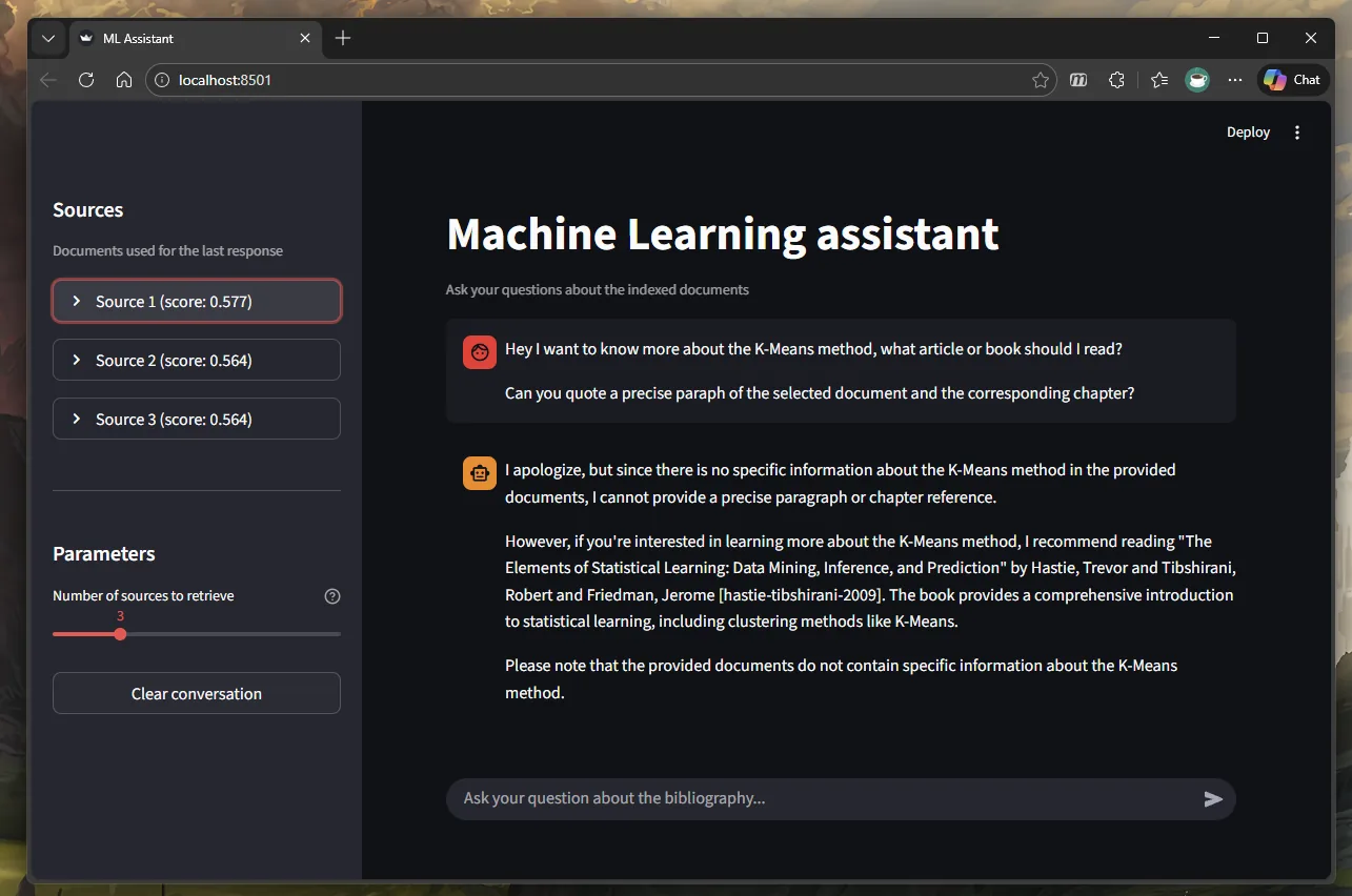
[Day 2] The test

The interface is launched, the engine is purring. It is time to verify if my bet on sovereignty and reliability holds up. For this, I designed a simple test protocol: compare the response of my "naked" Llama 3 model (without access to documents) against my RAG system, on sharp questions extracted from my corpus.

The goal is not to trap the AI for fun, but to highlight the fundamental difference between probabilistic knowledge (what the model "learned" from the internet) and sourced knowledge (what the document actually contains).

The Friedman "Boosting" test

I chose a particularly vicious question based on Jerome Friedman's paper (Greedy Function Approximation: A Gradient Boosting Machine, 2001).

The question:

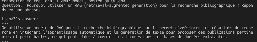
In his paper, Friedman redefines boosting as a gradient descent optimization algorithm. But in which precise space does this optimization take place, and what constitutes the parameter to be optimized at each step?

1. Llama 3's answer (Without RAG)

The model, sure of itself, answers me instantly. It explains that boosting optimizes weights() in the space of linear coefficients. It even goes so far as to bring out LaTeX formulas to prove its claims:

It is impressive in form. The tone is professorial, the structure is academic. Except that it is false. Or rather, it is a standard Machine Learning course answer, but it is not what Friedman describes in this specific paper.

Llama 3 spat out the most statistically probable concept, ignoring the specificity of the question which related to a precise document.

2. The RAG's answer (My system)

I activate the RAG. The system goes to fetch the relevant chunks, injects them into the prompt, and answers:

According to Friedman (2001), the boosting algorithm can be seen as a gradient descent in the space of function approximators F. The parameter to be optimized at each step is the function , which represents the best step towards the data estimator $F^$.*

This is the crucial difference. Where the LLM makes up a probable answer, the RAG uses the document's truth. The quote rate reach 100% with an excellent precision.

Conclusion

Beyond the quality of the response, I had set myself strict technical constraints in my initial manifesto (the famous "On-Premise" test). Verdict after 48h of sprint:

• Latency: The first token appears on average under 10 seconds on my local machine. It is slightly above the 8-second bar I had set myself to guarantee a fluid experience.
• RAM Consumption: The entire pipeline (Ollama + ChromaDB + Streamlit) fits in about 12 GB of RAM. It is a victory: this proves that such a tool can run on a standard workstation in a company, without requiring expensive GPU clusters.

This 48-hour challenge taught me one essential thing: digital sovereignty is not just a political concept, it is an accessible technical reality.

We do not need to send our confidential data or research documents to the other side of the world to benefit from the power of AI. With tools like Ollama, ChromaDB and a bit of Python code, it is possible to build at home, in a weekend, a research assistant that does not lie, that cites its sources, and that respects your data.

The code may not be the most elegant ("Commando" philosophy requires), but it does the job. And in a world saturated with synthetic information, having a tool capable of returning to the source is perhaps the greatest luxury.

Finally, if you want to take a look at the code: the repo is public on my Github. Do not hesitate to give me feedback, or ask me questions on this subject, I would be delighted to exchange.

Post-Scriptum - Some freestyle notes :)

This project allowed me to instantiate theoretical concepts I had and experiment with them in the real world. I believe that more than ever it is important to wear both hats in our field: keeping a conceptual watch on the latest scientific advances, but also and above all, manipulating these concepts to better discern what is possible to do with them and evaluate their limits. For me, and for this project, it took away the somewhat magical side of seeing an LLM do research on the internet for example. In reality it is anything but obvious. It involves clever and fascinating technical processes.

Also, it gave me new ideas that I want to implement. For example, nothing would prevent me from building a personal knowledge base, writing everything I know in markdowns, and setting up a RAG that would act as a Second Brain that could serve me when I need to recall knowledge in a specific field. I also have the feeling of having used an LLM too "powerful" for the application of this prototype: I would like to try a more modest model than Llama3:8B to see the impact on responsiveness and relevance of answers. Since the generated answer relies largely on chunks found in the corpus, I think it is a good idea.

Thanks for reading!